Supplementary Material: Parameter Sensitivity of Deep-Feature based Evaluation Metrics for Audio Textures

submitted to ISMIR 2022

1 Gram-Matrix - details

1.1 Gram-Matrix Computation

The Gram-matrix for the $n^{th}$ CNN is computed as the time-averaged correlations between the feature maps from the filters. Specifically, each element of the Gram-matrix of the $n^{th}$ CNN is defined as

G_{pq}^{n} = \sum_{m = 1}^{M} f_{pm}^{n} \cdot f_{qm}^{n} = f_{p}^{n} \cdot {(f_{q}^{n})}^{T}

(1)

where, $M$ is the total number of time frames, $f_{p}$ and $f_{q}$ are the feature maps of dimension $1 \times M$ of the $p^{th}$ and the $q^{th}$ filters, where $p$ and $q$ range from 1 to the number of filters, $F$ , i.e. 512. The resulting Gram-matrix, thus, has dimensions $512 \times 512$ at the output of each CNN, and the Gram-matrix of the $n^{th}$ CNN consists of dot products of the feature maps, written as,

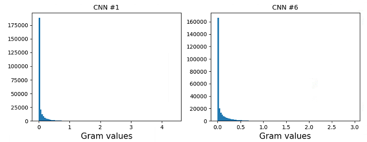
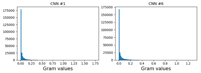
\begin{matrix} G = [\begin{matrix} ⟨ f_{1}, f_{1} ⟩ & ⟨ f_{1}, f_{2} ⟩ & . . & ⟨ f_{1}, f_{F} ⟩ \\ ⟨ f_{2}, f_{1} ⟩ & ⟨ f_{2}, f_{2} ⟩ & . . & ⟨ f_{2}, f_{F} ⟩ \\ . . . \\ ⟨ f_{F}, f_{1} ⟩ & ⟨ f_{F}, f_{2} ⟩ & . . & ⟨ f_{F}, f_{F} ⟩ \end{matrix}] & (2) \end{matrix}

1.2 Sparsity of Gram-Matrix

Figure 1 shows the histogram of the values of the Gram matrices from the first ( $k_{1} = 2$ ) and the sixth ( $k_{6} = 128$ ) CNNs from a Frequency Modulation (FM) signal at a particular carrier frequency, modulation frequency, and modulation index and a water-filling sound at a particular fill level in a container. Although the range of values in these Gram-matrices are different (x-axis), it is evident from the histograms of the Gram-matrices of both these textures that they are sparse with most values of the matrix being close to zero. This suggests that non-zero values of the correlation between feature maps are sparsely located.

Figure 1:Histogram plots of the values of Gram-matrices from the first (k=2) and the sixth (k=128) CNNs. The top two plots are from a frequency modulation (FM) texture and the bottom two plots are from a water-filling texture.

1.3 Gram Vector Computation

We divide each row of the Gram matrix from equation 2 into segments of length $s$ , as shown in equation 3, where in our experiments, we use $s = 128$ .

\begin{matrix} G = [\begin{matrix} ⟨ f_{1}, f_{1} ⟩ & ⟨ f_{1}, f_{2} ⟩ & . . & ⟨ f_{1}, f_{s} ⟩ & . . . . . . . & ⟨ f_{1}, f_{F} ⟩ \\ ⟨ f_{2}, f_{1} ⟩ & ⟨ f_{2}, f_{2} ⟩ & . . & ⟨ f_{2}, f_{s} ⟩ & . . . . . . . & ⟨ f_{2}, f_{F} ⟩ \\ . . . \\ ⟨ f_{F}, f_{1} ⟩ & ⟨ f_{F}, f_{2} ⟩ & . . & ⟨ f_{F}, f_{s} ⟩ & . . . . . . . & ⟨ f_{F}, f_{F} ⟩ \end{matrix}] & (3) \end{matrix}

The Gram vector of dimension $1 \times s$ is computed as a row aggregated average vector over all the Gram matrices of a given audio texture. The first element of the Gram vector of the Gram-matrix from the $n^{th}$ CNN is computed as

g_{1}^{n} = \frac{1}{4} \cdot \frac{1}{F} (\sum_{i = 1}^{F} ⟨ f_{i}, f_{1} ⟩ + \sum_{i = 1}^{F} ⟨ f_{i}, f_{s + 1} ⟩ + \sum_{i = 1}^{F} ⟨ f_{i}, f_{2 s + 1} ⟩ + \sum_{i = 1}^{F} ⟨ f_{i}, f_{3 s + 1} ⟩)

(4)

Similarly, the last element of this vector for the Gram-matrix from the $n^{th}$ CNN is computed as,

g_{s}^{n} = \frac{1}{4} \cdot \frac{1}{F} (\sum_{i = 1}^{F} ⟨ f_{i}, f_{s - 1} ⟩ + \sum_{i = 1}^{F} ⟨ f_{i}, f_{2 s - 1} ⟩ + \sum_{i = 1}^{F} ⟨ f_{i}, f_{3 s - 1} ⟩ + \sum_{i = 1}^{F} ⟨ f_{i}, f_{4 s - 1} ⟩)

(5)

Therefore, the overall gram vector $g$ of dimension $1 \times s$ is the element-wise mean of these vectors over the $N$ Gram matrices of an audio texture corresponding to the CNNs, given as

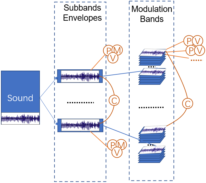
\begin{matrix} g = [\begin{matrix} \frac{1}{N} \sum_{n = 1}^{N} g_{1}^{n} & \frac{1}{N} \sum_{n = 1}^{N} g_{2}^{n} & . . . & \frac{1}{N} \sum_{n = 1}^{N} g_{s}^{n} \end{matrix}] & (6) \end{matrix}

2 Cochlear Param-Metric (CPM) - details

The implementation uses a cochlear filterbank with 36 Gammatone filters, with Hilbert transform to compute the envelopes, and then compresses the envelopes with an exponential rate of 0.3 on each element in the matrix [1]. The modulation filterbank with 20 filters is applied on each envelope, thus generating 36 $\times$ 20 modulation bands.

For each sound $x$ , seven sets of statistics are computed, denote them by $S^{i}$ where $i = [1 . . . 7]$ ,

Sub-band envelope power: average of the square sum, 36 $\times$ 1.
Sub-band envelope marginal statistics: mean, variance, skewness, kurtosis, 36 $\times$ 4.
Sub-band envelope variance: 36 $\times$ 1.
Sub-band envelope correlations: the correlation between each envelope, 36 $\times$ 36.
Modulation power: average of the square sum of each modulation bands, 36 $\times$ 20.
Modulation variance: 36 $\times$ 20.
Modulation correlation: the correlation between the same modulation bands for every 2-step nearest envelopes, in total (36 $\times$ 5-6) $\times$ 20 = 3,480.

The algorithm, thus, generates 6,432 statistical parameters.

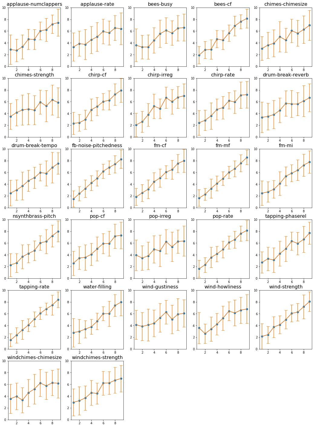
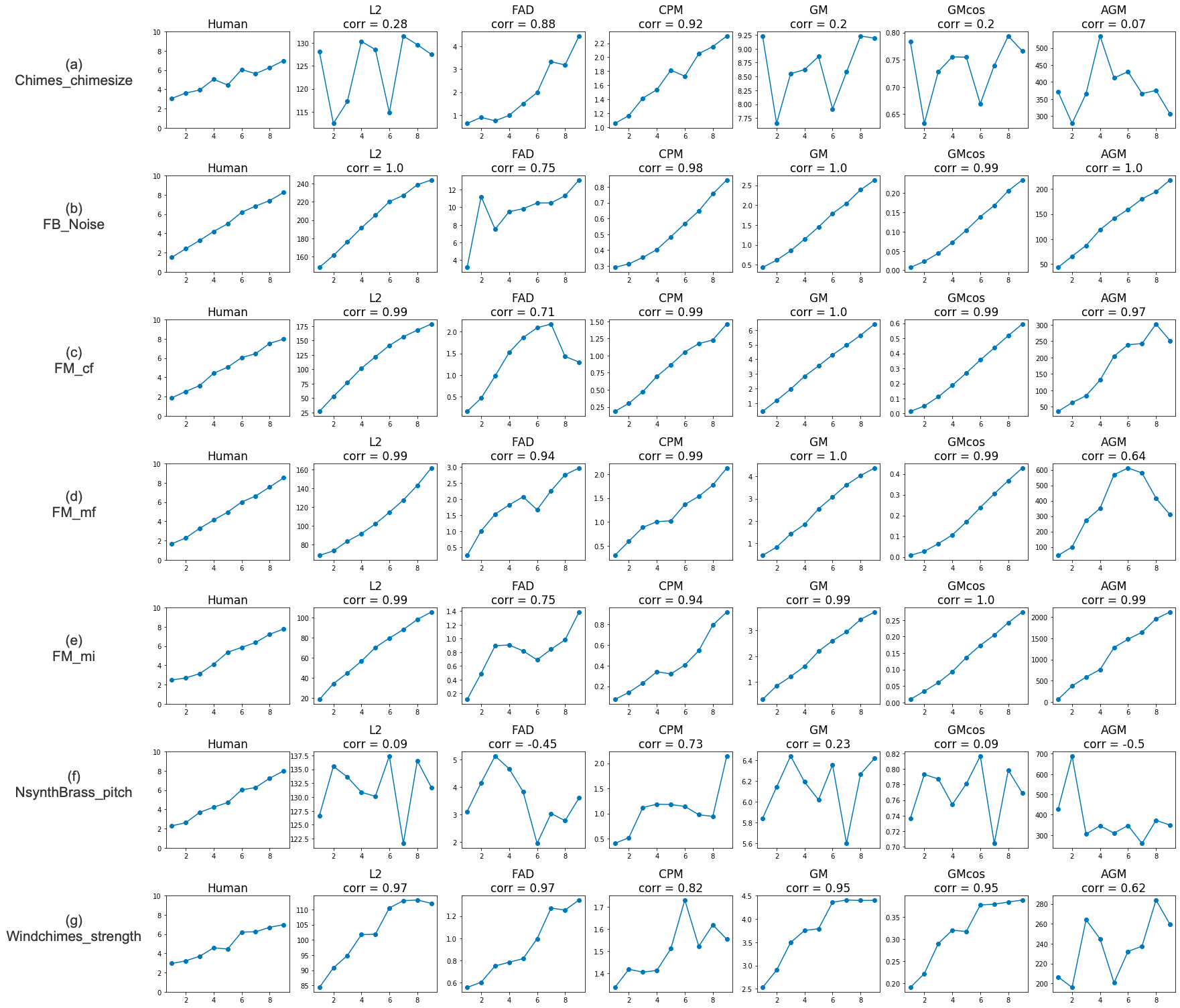
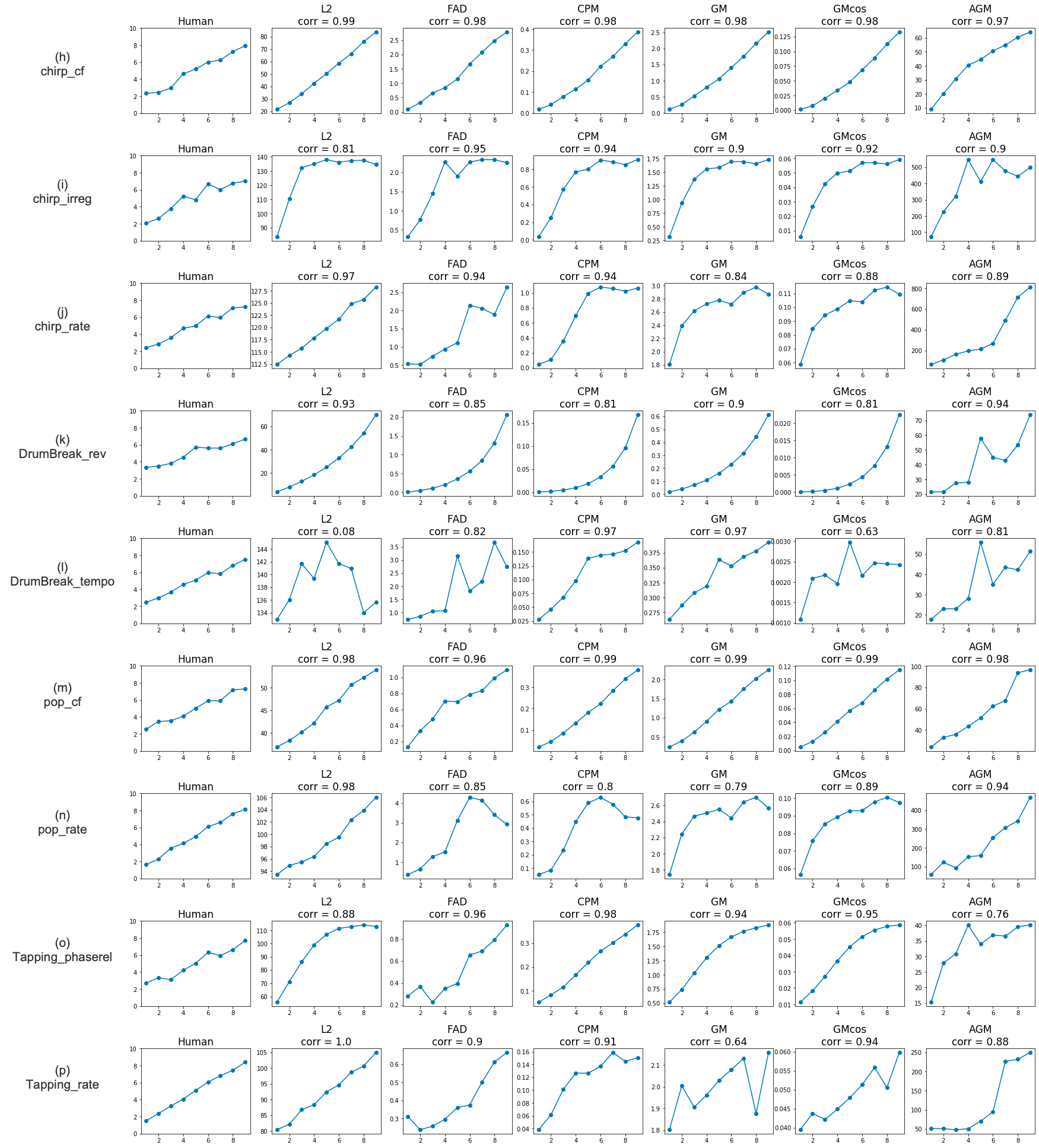
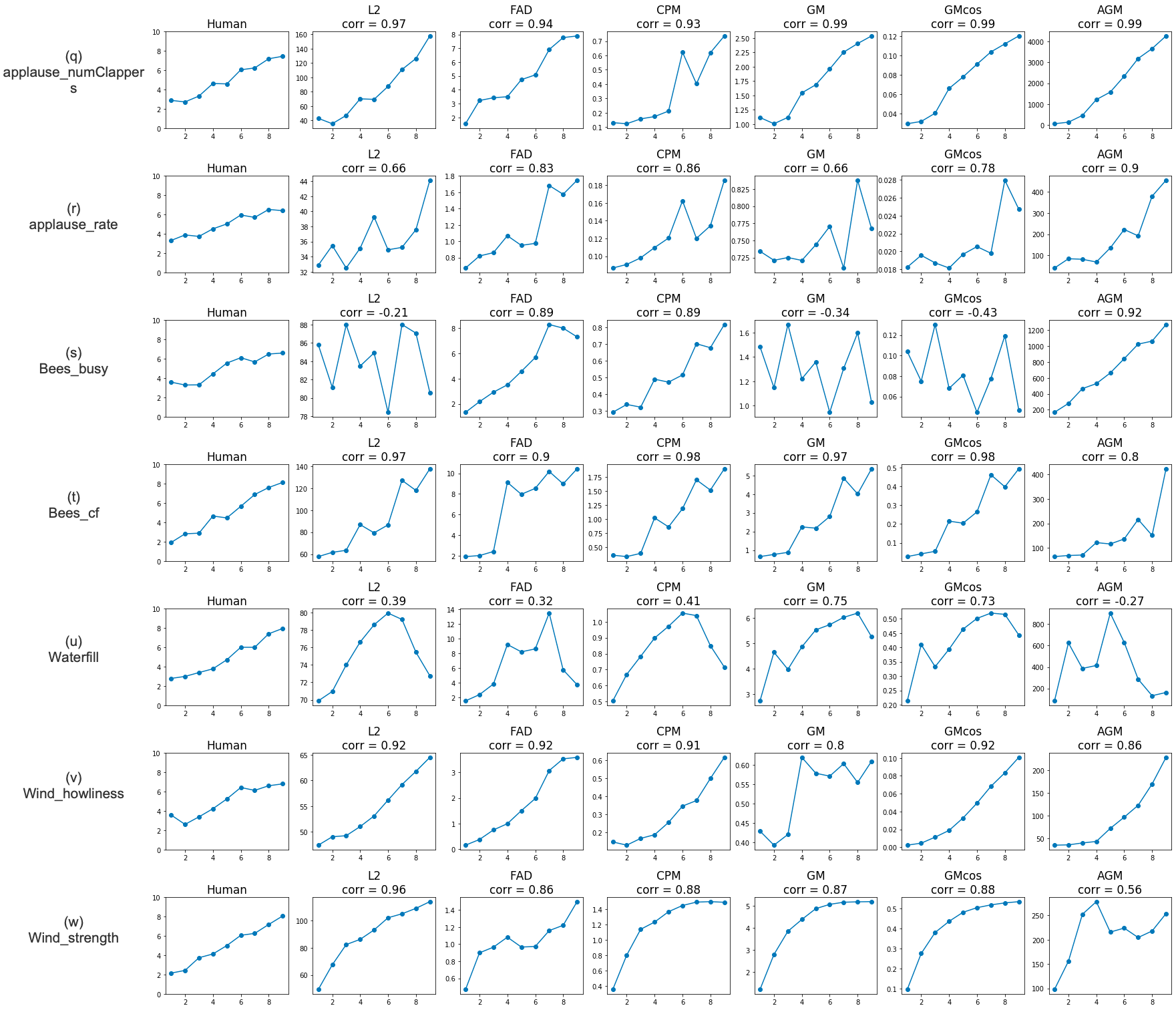
Figure 2:CPM from the statistics derived from Mc Dermott and Simoncelli (2011). Red icons denote the statistical measurements: P: power, M: marginal statistics, V: variance, C: correlations between subbands as described above.

3 Comparison plots for objective metrics with human perceptual measures

The trends of subjective responses and objective metrics can be observed for the three sets of audio textures in Figures 3 (pitched), 4 (rhythmic), and 5 (others).

Figure 3:Comparison plots for pitched sounds

Figure 4:Comparison plots for rhythmic sounds

Figure 5:Comparison plots for other sounds

4 Human Listening Test Plots

The rank-order responses obtained from the human listening tests are plotted in Figure 6.

Figure 6:Plots showing rank orders captured from human listening tests (y-axis) w.r.t control parameter (x-axis) used to generate the audio samples. Error bars show the standard deviation of the ranks collected at each control parameter.

References

[1] Josh H McDermott and Eero P Simoncelli. Sound texture perception via statistics of the auditory periphery: evidence from sound synthesis. Neuron, 71(5):926–940, 2011.